From Slicer to MATLAB: a Segmentation Workflow

You have segmented some anatomy in 3D Slicer. Now what? This page walks through the whole path from a Slicer segmentation to measurements, comparisons, and class statistics in MATLAB. It follows the SLCR live scripts in Unit 3, and each step tells you which script covers it in detail.

Each step has a picture of the result, the few lines of code that make it, and a link to the MtM Toolbox page for the full details of each function.

flowchart TD
    A["1. Segment in Slicer<br/>save .seg.nrrd"] --> B["2. Load in MATLAB<br/>medicalVolume"]
    B --> C["3. Display<br/>2D and 3D"]
    C --> D["4. Pull out one segment<br/>voxels to mm"]
    D --> E["5. Measure<br/>volume, length, diameter"]
    D --> F["6. Compare two<br/>segmentations"]
    F --> G["7. Compare left<br/>and right"]
    E --> H["8. Compare a<br/>whole class"]
    G --> H

Step	What you do	Main functions	Live script
1	Segment and save in Slicer	Segment Editor	CTACardio, CT Femur
2	Load the CT and the segmentation	medicalVolume, mmGetSlicerSegmentInfo, mmMatchVolumeGeometry	SLCR1, SLCR2
3	Display in 2D and 3D	labeloverlay, volshow, mmPlotAllSeg	SLCR1
4	Pull out one segment, in mm	mmGetMedicalVolumeSegment, mmPlotMask2Surface	SLCR1, SLCR2
5	Measure volume, length, and diameter	regionprops3, mmAlignSurface2Axes, mmCrossSectionProfile	SLCR4
6	Compare two segmentations	dice, mmSurfaceDistance	SLCR2, SLCR3
7	Compare left and right	mmMirrorAlign, mmSurfaceDistance	SLCR5
8	Compare the whole class	mmGetSlicerSegmentInfoAll, mmBoxSwarm	SLCR5, SLCR6

Before you start

• Add the MtM toolbox to your MATLAB path (see the setup page)
• You need the Medical Imaging Toolbox and the Image Processing Toolbox
• Get the SLCR live scripts with mmGetScript(3)

1. Segment and save in Slicer

Segment your structures in the Segment Editor, following the CTACardio or CT Femur tutorial. Then save your work (File → Save Data). Slicer saves two files that MATLAB needs:

• the intensity volume (the CT or MRI), as a .nrrd file. For example, CTACardio Crop.nrrd
• the segmentation, as a .seg.nrrd file. For example, Salcedo Segmentation.seg.nrrd

The kidneys segmented in Slicer. Each segment has a name and a color, and Slicer stores both in the .seg.nrrd file.

Name your segments and files carefully

MATLAB finds segments by name, so use the names in the tutorial ("right kidney", "left femur"). Start the file name with your last name and a space (Salcedo Segmentation.seg.nrrd): in step 8, the part before the space becomes your ID.

2. Load the volumes in MATLAB

Load both files as medicalVolume objects. A medicalVolume holds the voxels and the geometry of the volume: its voxel size, orientation, and position in the patient. Then read the segment names, label values, and colors with mmGetSlicerSegmentInfo.

folder = fullfile(mmSetUnitDataFolder(3), "CTACardio");
ctMV = medicalVolume(fullfile(folder, "CTACardio Crop.nrrd"));                  % CT
segMV = medicalVolume(fullfile(folder, "Salcedo Segmentation.seg.nrrd"));       % segmentation
segT = mmGetSlicerSegmentInfo(fullfile(folder, "Salcedo Segmentation.seg.nrrd"))

segT

       SegName        Layer    LabelValue                Color
    ______________    _____    __________    _____________________________
    "right kidney"      1          1         0.56471    0.93333    0.56471
    "left kidney"       1          2               0    0.59216    0.80784
    "aorta"             1          3         0.84706    0.39608     0.3098

Every voxel of segMV.Voxels holds a label value: 0 for background, 1 for the right kidney, 2 for the left kidney, and 3 for the aorta.

Is the segmentation the same size as the CT?

Some versions of Slicer add an empty slice to a segmentation. Then MATLAB can't compare it voxel by voxel with the CT. mmMatchVolumeGeometry adds or removes the extra slices, so the two line up:

segMV = mmMatchVolumeGeometry(segMV, ctMV);

3. Display the segmentation

Check your segmentation before you measure it. First, overlay one slice of the segmentation on the CT, in the segment colors from Slicer:

ctSlice = extractSlice(ctMV, 90, "transverse");
labelSlice = extractSlice(segMV, 90, "transverse");
imshow(labeloverlay(mat2gray(ctSlice, [-160 240]), labelSlice, Colormap=segT.Color, Transparency=0.3))

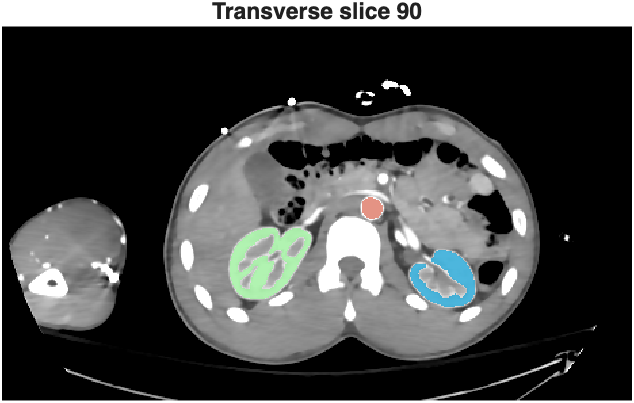
A transverse slice through both kidneys, with the segmentation in the Slicer colors.

Then look at it in 3D. volshow renders the CT and the segmentation together. mmPlotAllSeg turns every segment into a surface:

viewer = viewer3d(BackgroundColor="white", BackgroundGradient="off");
volshow(ctMV, Parent=viewer, RenderingStyle="GradientOpacity", OverlayData=segMV.Voxels);

figure
mmPlotAllSeg(segMV, segT);

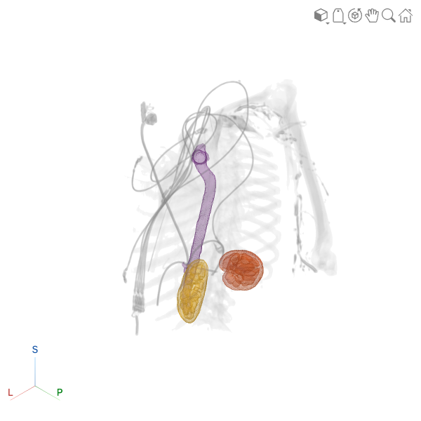
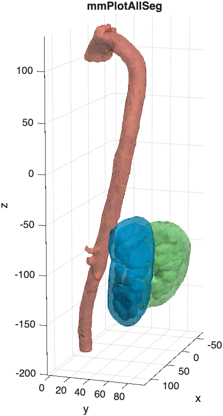
Left: volshow with the segmentation as an overlay. Right: mmPlotAllSeg plots each segment as a surface, in its Slicer color.

4. Pull out one segment

Most analyses work on one structure at a time. mmGetMedicalVolumeSegment returns a structure with the mask of one segment, its color, and tform: the transformation that converts voxel positions to millimeters in the patient. Use tform whenever you make a surface, so that your measurements are in mm, not voxels.

rk = mmGetMedicalVolumeSegment(segMV, segT, segName="right kidney")
mmPlotMask2Surface(rk.mask, fcolor=rk.color, transform=rk.tform);

rk

    segName: "right kidney"
       mask: [465×276×390 logical]
      color: [0.5647 0.9333 0.5647]
      tform: [1×1 affinetform3d]
    spacing: [1.027 1.027 1.027]
     volume: 99574

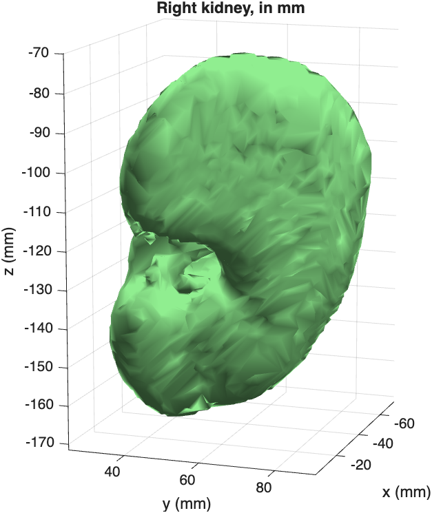
The right kidney as a surface. The axes are in mm, because the surface was transformed with rk.tform.

volume is in voxels

Multiply by the volume of one voxel to get mm³: rk.volume * prod(segMV.VoxelSpacing). Divide by 1000 for mL. For this kidney, that's 108 mL.

5. Measure

Volume and mean intensity

regionprops3 measures every segment at once. Turn the label volume into a categorical array first, so the rows are named after the segments:

segCat = categorical(segMV.Voxels, segT.LabelValue, segT.SegName);
rp = regionprops3(segCat, ctMV.Voxels, "Volume", "MeanIntensity");
rp.Volume_mL = rp.Volume * prod(segMV.VoxelSpacing) / 1000

Length

SLCR4 measures the femurs of donor 9553F. To measure the length of a bone, center its surface, turn its long axis upright with mmAlignSurface2Axes, and measure its range along z:

rSeg = mmGetMedicalVolumeSegment(segMV, segT, segName="right femur");
hp = mmPlotMask2Surface(rSeg.mask, fcolor=rSeg.color, smooth=true, transform=rSeg.tform);
v = mmAlignSurface2Axes(hp.Vertices - mean(hp.Vertices));   % long axis along x
hp.Vertices = mmRotateSurfaceVertices(v, 'y', 90);           % long axis along z
femurLength = range(hp.Vertices(:,3))                        % mm

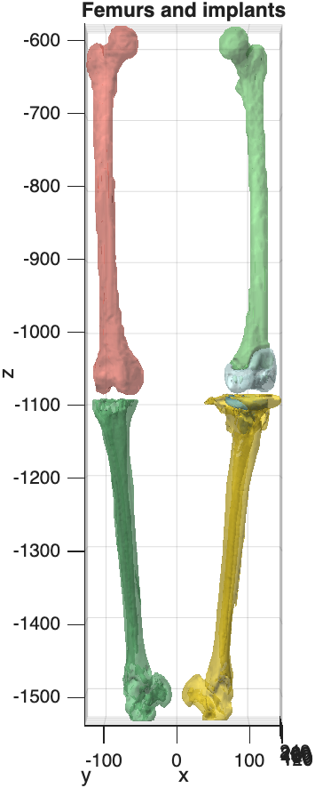
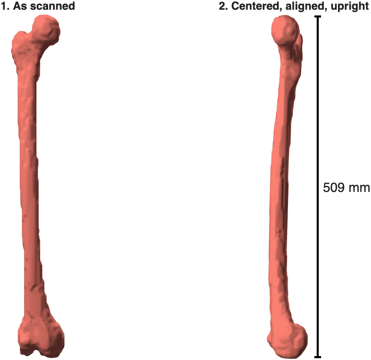
Left: the femur segmentation of donor 9553F, with a hip implant in the left femur. Right: the right femur, centered and aligned. Its length is 509 mm.

Diameter along the length

mmCrossSectionProfile cuts a bone or vessel into thin slabs, perpendicular to its long axis, and measures every slab: its area, its equivalent diameter, and its narrowest and widest widths.

[profileT, info] = mmCrossSectionProfile(rSeg, Title="Right femur");
info.At          % the cross-section at midshaft (50% of the length)

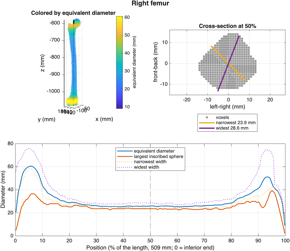
The femur colored by diameter (top left), the cross-section at midshaft with its narrowest and widest widths (top right), and the diameter profile from the knee (0%) to the hip (100%).

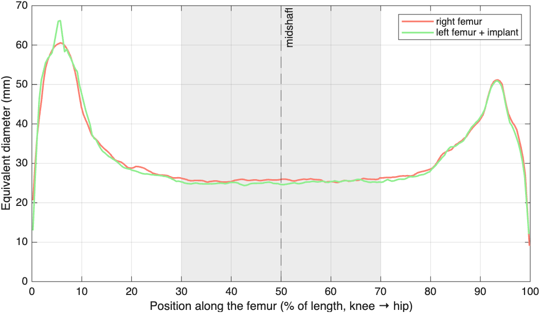
Plot two profiles together to compare bones. The implant hardly changes the diameter of the left femur:

Curved structures

For a curved vessel like the aorta, use Centerline="curved". The function then follows the middle of the vessel instead of a straight axis. Try it in the challenge at the end of SLCR4.

6. Compare two segmentations

How well do two segmentations of the same structure agree? In SLCR2 you compare your kidney with the kidney from TotalSegmentator. In SLCR3 you compare two segmentations of the same tumor.

Where do they overlap?

The Dice coefficient measures the overlap: 1 is a perfect match, 0 is no overlap. To see where they differ, color each voxel by which segmentation it belongs to:

mySeg = mmGetMedicalVolumeSegment(segMV, segT, segName="right kidney");
totSeg = mmGetMedicalVolumeSegment(totalMV, totalT, segName="right kidney");
dice(mySeg.mask, totSeg.mask)      % 0.78

compare = zeros(size(mySeg.mask), "uint8");
compare(mySeg.mask & totSeg.mask) = 1;      % both (green)
compare(totSeg.mask & ~mySeg.mask) = 2;     % TotalSegmentator only (cyan)
compare(mySeg.mask & ~totSeg.mask) = 3;     % ours only (magenta)

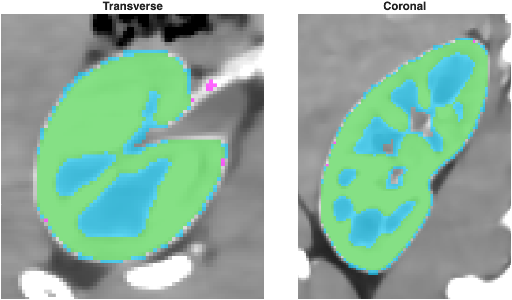
Green: in both segmentations. Cyan: only in TotalSegmentator's. Our kidney leaves out the renal sinus (the cyan areas inside), which TotalSegmentator fills in.

How far apart are the surfaces?

mmSurfaceDistance measures, for every point on one surface, the distance to the other surface: negative (blue) if the point is inside the other segmentation, positive (red) if it is outside. The table summarizes the distances.

T = mmSurfaceDistance(mySeg, totSeg, Names=["Ours" "TotalSegmentator"])

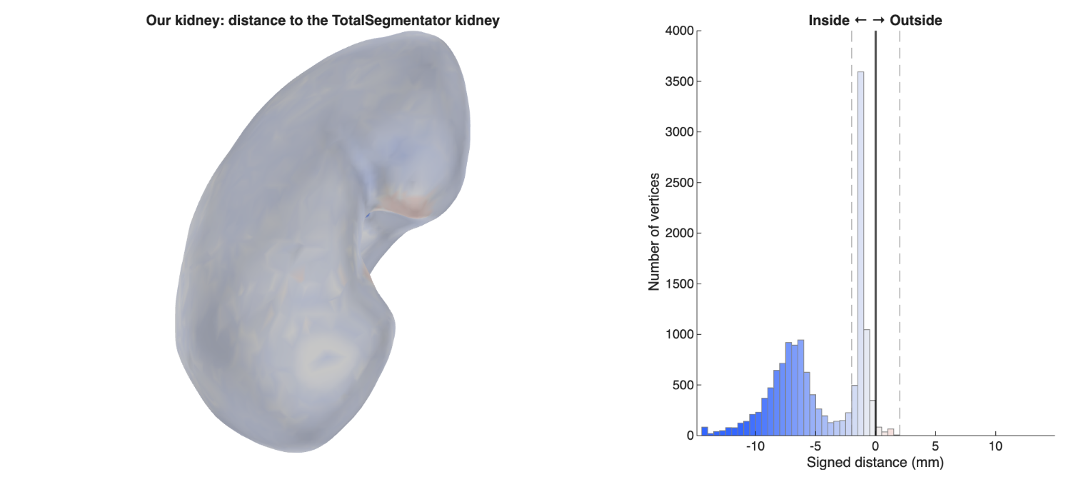
The outside of our kidney agrees with TotalSegmentator's (white). The blue peak in the histogram, 5–10 mm inside, comes from the surfaces of the holes inside our kidney. SLCR2 shows how to fill them.

When neither segmentation is the reference, as with the two tumor segmentations in SLCR3, measure in both directions:

T = mmSurfaceDistance(t1Seg, t2Seg, Names=["Tumor1" "Tumor2"], Direction="both")

Top: Tumor1 measured against Tumor2. Bottom: Tumor2 measured against Tumor1. More than 90% of both surfaces are within 2 mm of each other (Dice 0.93).

7. Compare left and right

Are the left and right kidneys the same shape? To compare them, mmMirrorAlign flips the left kidney across the midline, then rotates and moves it until it fits the right kidney as closely as possible. Now both are on the same voxel grid, and you can compare them like two segmentations of the same structure.

rk = mmGetMedicalVolumeSegment(segMV, segT, segName="right kidney");
lk = mmGetMedicalVolumeSegment(segMV, segT, segName="left kidney");
[lkOnRk, rmse] = mmMirrorAlign(rk, lk);
mmSurfaceDistance(rk, lkOnRk, Names=["Right kidney" "Left kidney (mirrored)"], Direction="both")

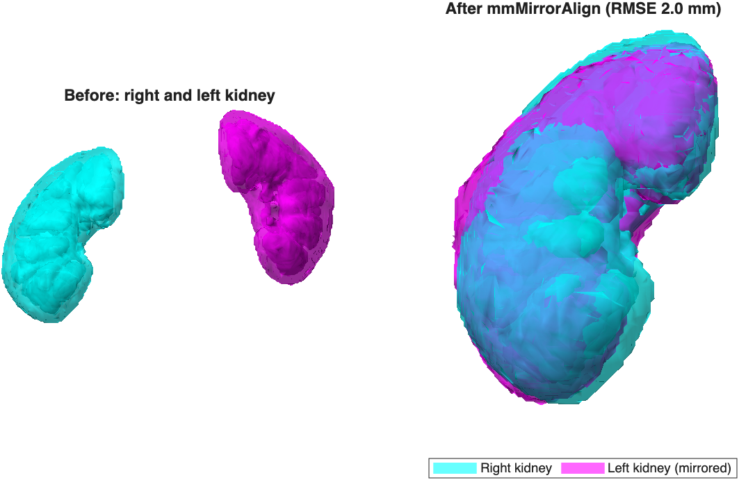
Before: the two kidneys where they sit in the body. After: the left kidney, mirrored and aligned on the right kidney.

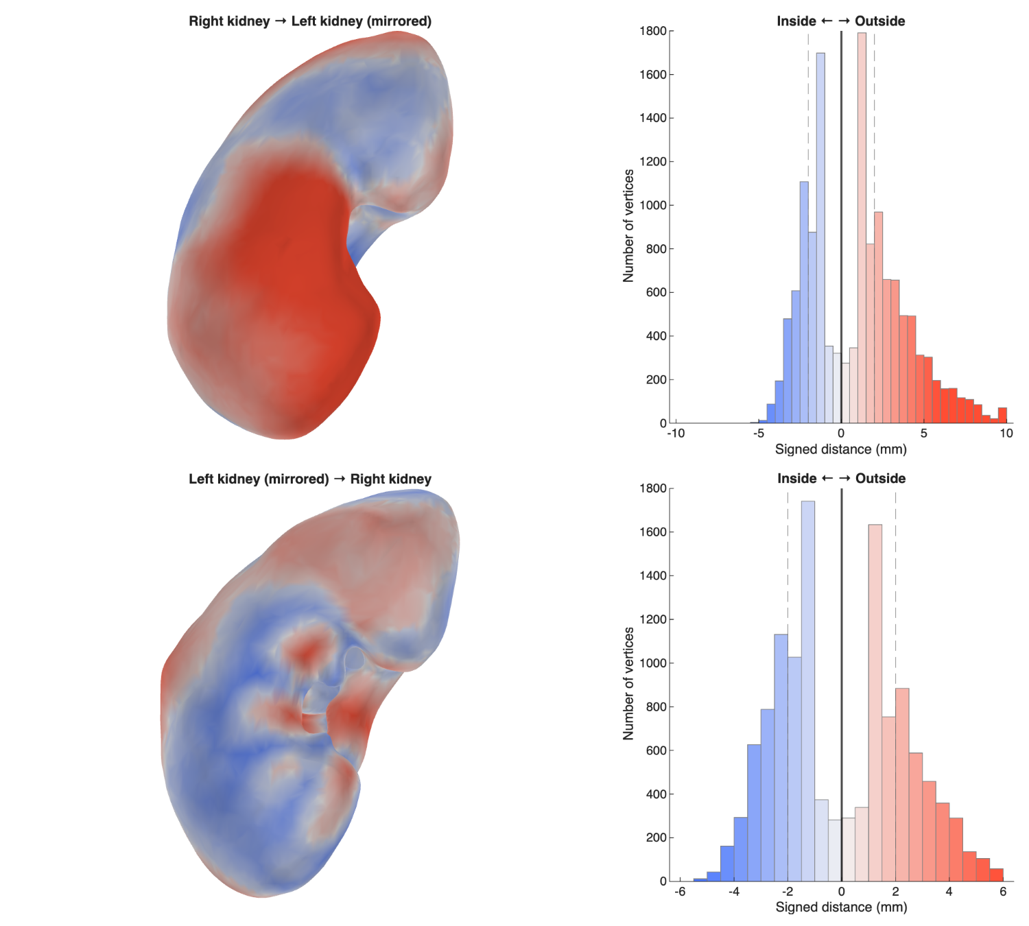
The right kidney is mostly outside the mirrored left kidney (red): in this donor, the right kidney is larger.

8. Compare a whole class

One segmentation is one opinion. With everyone's segmentations of the same scan, you can ask two new questions: how much do the raters disagree, and is a left–right difference bigger than that disagreement?

The figures in this step use made-up class data

The ten "students" below are fake segmentations, each with a typical mistake built in. Your class results will look different.

Load every file in a folder

Put everyone's .seg.nrrd files in one folder. mmGetSlicerSegmentInfoAll reads all of them, and takes each student's ID from the start of the file name:

[classSegT, contentT] = mmGetSlicerSegmentInfoAll(classFolder);
groupsummary(classSegT, "SegName")      % did everyone name their segments the same way?

Then measure each file in a loop. Wrap each file in try/catch, so that one bad file doesn't stop the loop. The local functions in SLCR5 and SLCR6 (measureKidneys, loadFemur) also fix common mistakes, like swapped left and right labels or names in capital letters.

kidneyT = table();
for k = 1:height(contentT)
    file = fullfile(contentT.folder(k), contentT.name(k));
    try
        kidneyT = [kidneyT; measureKidneys(file, contentT.ID(k))];
    catch err
        warning("%s: %s", contentT.ID(k), err.message)   % skip this file
    end
end

Look for mistakes first

Before you calculate anything, look at every segmentation. Mistakes are easy to see in a gallery:

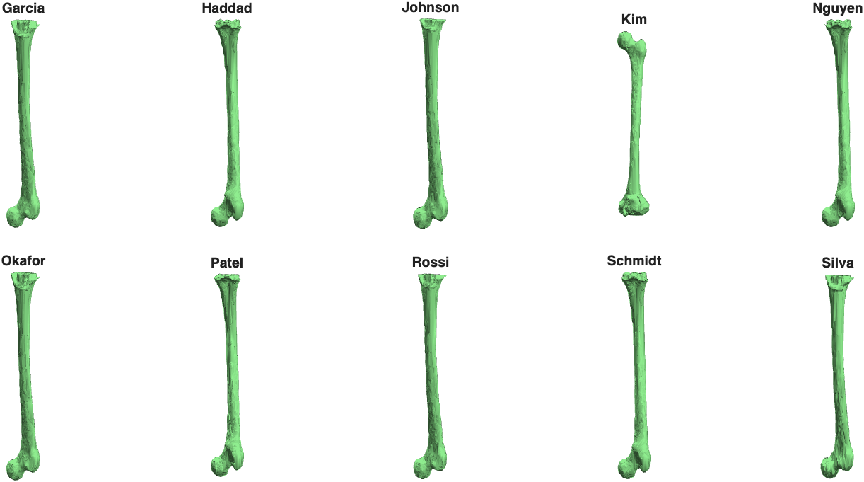
The left femur of each (made-up) student. Kim forgot to cut the femur at the base of the implant, so the whole femur is included. Kim's left femur is 40 mm longer than everyone else's, and it shows up as an outlier in the next plot.

Plot the class

mmBoxSwarm draws a box chart with each measurement as a point on top, so you can see every student and the spread at once:

mmBoxSwarm(femurT.Side, femurT.Length_mm);

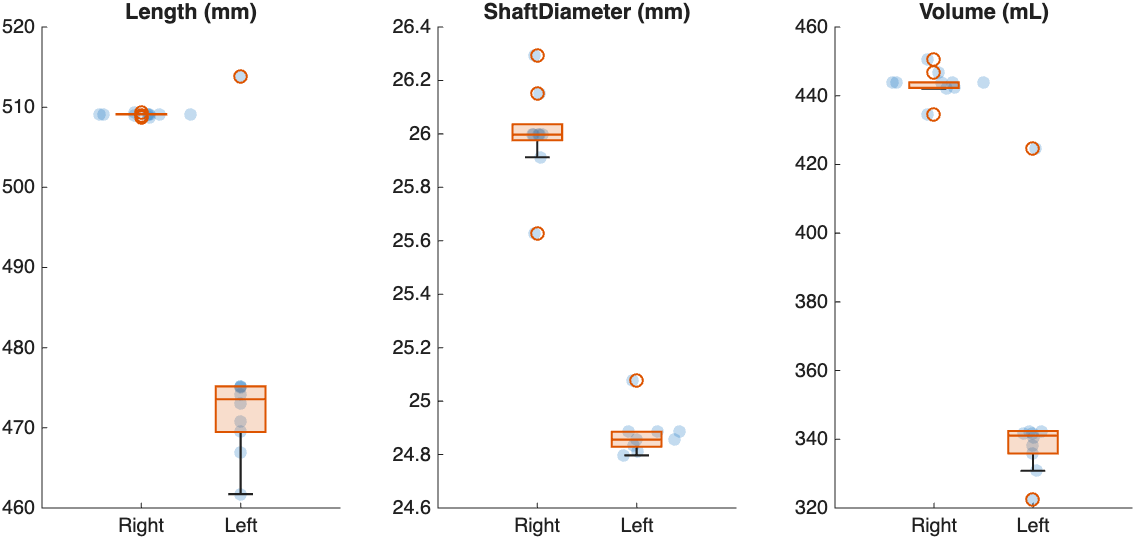
Femur length, shaft diameter, and volume for each student. The right femur (segmented automatically) barely varies. The left femur (cut by hand) varies more, and Kim's femur is the outlier at the top.

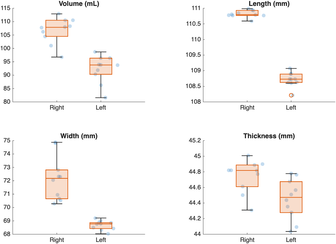
Kidney measurements for each student. Every student found the right kidney larger than the left.

How much do the raters disagree?

The coefficient of variation (CV) is the standard deviation between raters as a percent of the mean. Below 5% is good agreement. Above 10% is poor.

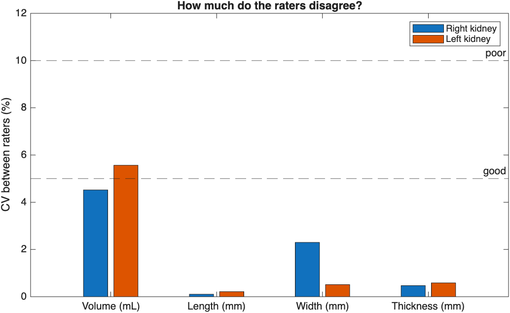
The raters agree closely on length, width, and thickness, but less on volume, which depends on every voxel at the edge.

Is the difference real?

Pair each student's right and left measurements. If every line slopes the same way, the difference is in the anatomy, not in the raters:

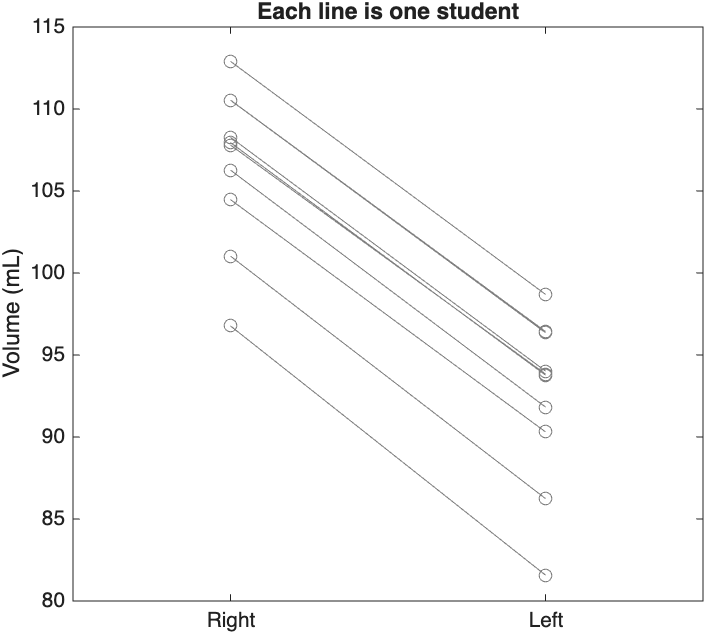
Each line is one student. Every student's right kidney is larger than their left. SLCR5 tests this with a signed-rank test, and compares the difference with the disagreement between raters.

Shortcut: let AI segment for you

Two toolbox functions segment scans without opening Slicer, so you can process many scans in a loop:

• mmTotalSegmentator segments a CT into more than 100 structures (see SLCR7)
• mmSynthSeg2 segments a brain MRI into 32 structures

Their output works with every step on this page, starting at step 2.