Distance Transform

How far is every pixel from the thing you care about?

Overview

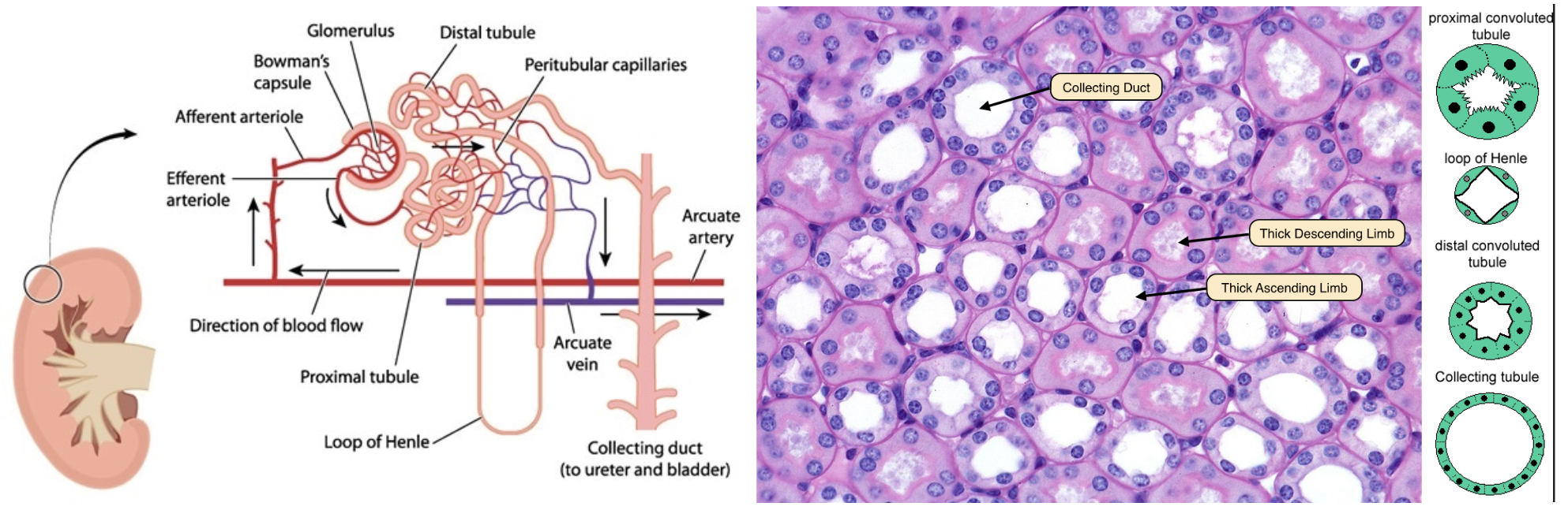
A cross-section through the kidney medulla cuts through several kinds of tubules. Two of them can look similar in an H&E section: the thin limbs of the loop of Henle, lined by flat cells with only a few nuclei, and collecting ducts, lined by cuboidal cells with many nuclei. To tell them apart automatically, we need to count the nuclei surrounding each tubule—which means identifying all the nuclei near a given duct, but none of the nuclei that belong to its neighbors. That requires a way to measure distance inside an image. This is exactly what the distance transform does.

The plan for this module:

1. Segment the nuclei and the duct lumens using k-means clustering (from Color Segmentation)
2. Use the distance transform to draw a ring of a fixed width around each duct
3. Count the nuclei that touch each ring
4. Classify each duct by how many nuclei it has, normalized by its size

Before we get to pixels, though, it's worth reviewing where "distance" comes from in the first place.

Things you should know

• Calculate the distance between two points using the Pythagorean theorem and hypot
• Explain what the distance transform (bwdist) measures, and what a zero in its output means
• Use imregionalmax to find the ridge lines exactly halfway between objects
• Explain how the watershed transform uses the distance transform to separate touching objects
• Threshold a distance transform to draw a ring of a specific width around a mask
• Use imreconstruct to keep only the objects in one mask that touch a marker in another
• Normalize a count (like nuclei touching a duct) by a size measurement (like perimeter) to make fair comparisons across objects of different sizes

Key Terminology you should know

• Euclidean distance: straight-line distance, calculated via the Pythagorean theorem
• Distance transform: an image where every pixel's value is its distance to the nearest TRUE pixel in a reference mask
• Regional maximum: a pixel (or connected region of pixels) whose value is higher than all of its immediate neighbors
• Morphological reconstruction: a technique that keeps whole objects in a mask image that are touched by a marker image, and discards the rest

Key Functions

• hypot: Square root of the sum of squares (the hypotenuse)
• diff: Differences between consecutive elements
• bwdist: Distance transform of a binary image
• imregionalmax: Regional maxima of an image
• imreconstruct: Morphological reconstruction
• bwconncomp: Find connected components in a binary image
• watershed: Watershed transform (used by the course function mmGetWatershed)

---

Measuring Distance Between Points

Consider a triangle with three vertices:

• (0,0)
• (3,0)
• (3,4)

We can represent these vertices in the matrix V, where column 1 holds the x-coordinates and column 2 holds the y-coordinates:

V = [0 0; 3 0; 3 4];

scatter(V(:,1),V(:,2),'filled');
xlabel('x'); ylabel('y')
grid on
axis([-1 9 -1 9])

We can use the patch function to fill in the triangle's interior, or face:

Fill the triangle

patch(V(:,1),V(:,2),'cyan','LineStyle',':')
text(1, 2.5, 'c = ?')

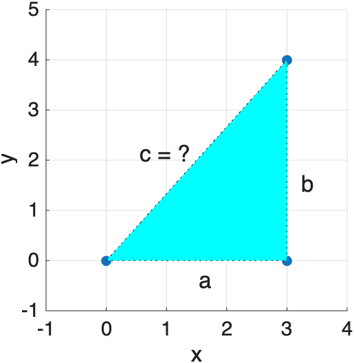
How long is the hypotenuse, c? The Pythagorean theorem gives us the answer, once we know the lengths of the two legs, a and b, which we can calculate from the x and y positions of the vertices.

a = 3-0; % length of a
b = 4-0; % length of b
c = sqrt(a^2+b^2) % length of c

result

c = 5

The function hypot does the same calculation in one step:

hypot

c = hypot(a,b) % c = 5

Distance Between Two Points

The same trick measures the straight-line (Euclidean) distance between any two points—just build the implied triangle:

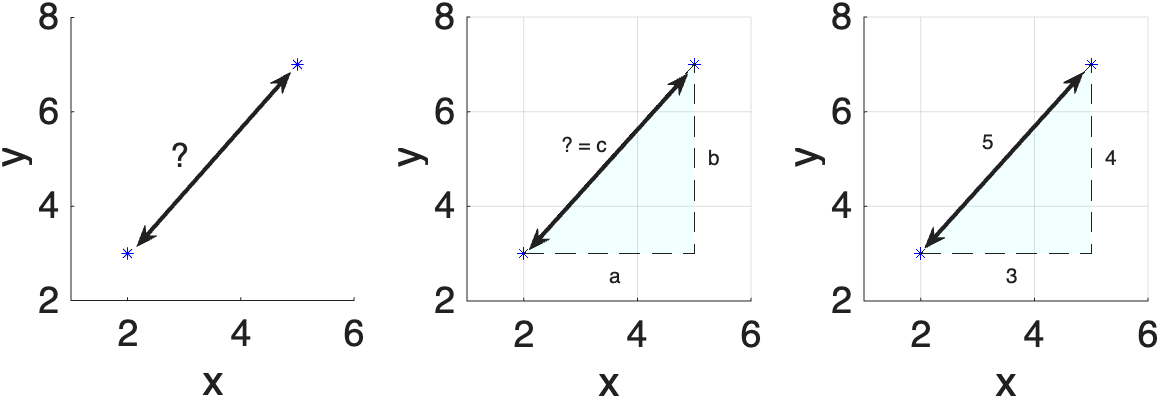
When measuring two points, visualize the triangle that the two points imply. Then, you just calculate a as the horizontal leg and b as the vertical leg of the triangle. With those two pieces of information, you then have enough information to calculate c, the hypotenuse and straight-line distance between your two points.

pts = [2 3; 5 7] % (2,3) and (5,7)

pts = 2×2
2   3
5   7

Calculate sides

sides = [5-2 7-3] % a and b sides

sides = 1×2
3   4

dist = hypot(sides(1),sides(2))

dist =

     5

Length of a Polyline

The same idea, repeated for every consecutive pair of points, gives the total length of a connected line:

pts = [0 0; 1 3; 2 1; 3 6; 4 7];

D = diff(pts);               % the sides of each segment's triangle
H = hypot(D(:,1), D(:,2));   % the length of each segment
L = sum(H)                   % total length

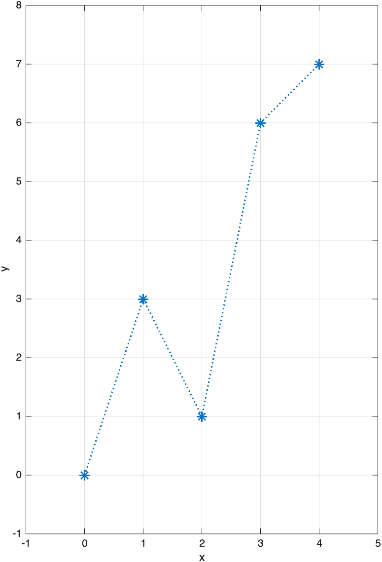
It really is "triangles all the way down": each segment of this zig-zagging line is the hypotenuse of its own small right triangle.

This also collapses into a single line of MATLAB math:

One-line distance formula

L = sum(sqrt(sum(diff(pts).^2,2)))

\[\text{Distance}=\sum_n \sqrt{\left(x_{n+1} -x_n \right)^2 +\left(y_{n+1} -y_n \right)^2 }\]

This formula—repeated distance-to-nearest-point calculations—is exactly what the distance transform does, except instead of a handful of named points, it does this for every single pixel in an image, all at once.

What Is the Distance Transform?

The distance transform replaces every pixel in a binary image with its distance (in pixels) to the nearest TRUE pixel. TRUE pixels themselves get a distance of 0. By default, bwdist measures straight-line (Euclidean) distance, so a diagonal neighbor is √2 ≈ 1.41 pixels away—exactly the Pythagorean calculation above, just automated for the whole image.

Consider a 5×5 logical array with a single TRUE at its center:

M = false(5);
M(3,3) = true;

B = bwdist(M);

result

B =
    2.8284    2.2361    2.0000    2.2361    2.8284
    2.2361    1.4142    1.0000    1.4142    2.2361
    2.0000    1.0000         0    1.0000    2.0000
    2.2361    1.4142    1.0000    1.4142    2.2361
    2.8284    2.2361    2.0000    2.2361    2.8284

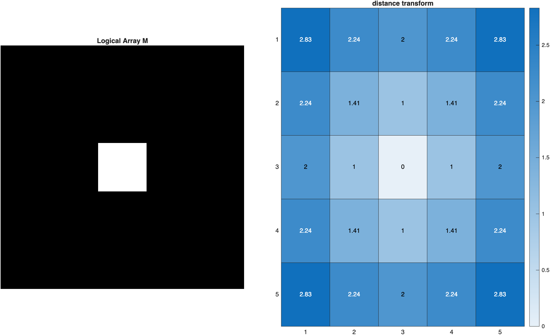
B is the same size as M. Every element contains the distance in pixels from that location to the nearest TRUE pixel. The location of the TRUE itself is zero, and diagonal neighbors are calculated with the Pythagorean theorem—just as we did by hand above.

Multiple TRUE Pixels

What happens with more than one TRUE pixel? Here we place four single points in a 100×100 array:

binmat = false(100);
binmat([2425 2475 7425 7475]) = true;

B2 = bwdist(binmat);
imshow(B2,parula(35))

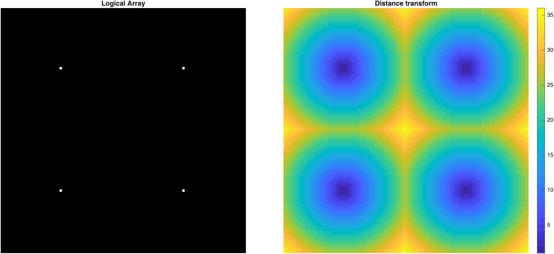
The distance transform is zero (dark) at each of the four points. Close to each point, the distance rings are circular, since every pixel measures its distance to its nearest TRUE. Where rings from neighboring points meet, they form straight lines exactly halfway between the points—so each point ends up "owning" one square quadrant of the image, with its rings morphing from circular near the center into a squared-off "squircle" as they approach the quadrant's edges. The largest distances (brightest) fall at the center and corners—the pixels farthest from any point.

Distance isn't always Euclidean

bwdist can measure distance several other ways by passing a method name as a second input: 'cityblock' (only horizontal/vertical steps), 'chessboard' (diagonal steps count the same as straight ones), and 'quasi-euclidean' (a fast Euclidean approximation). Applied to a single point, each produces a different shape instead of a circle:

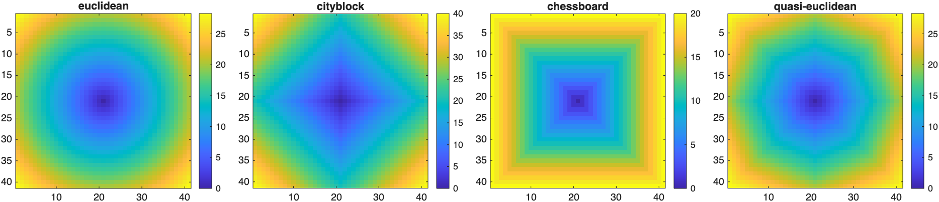
Euclidean gives a circle, cityblock gives a diamond, and chessboard gives a square—a nice reminder that "distance" is a choice, not just a fact about the pixels.

Distance Transform and the Watershed

So far, we have measured each pixel's distance to the TRUE pixels with bwdist(BW). If you invert the mask with ~, you get the opposite: bwdist(~BW) gives every pixel inside an object its distance to the nearest background pixel. The center of each object has the largest value, and the values fall off toward its edges. Where two objects touch, the distance dips at the narrow "neck" between them.

That dip is what lets us separate touching objects. The course function mmGetWatershed does this in three steps:

1. Distance transform. It computes bwdist(~BW) and inverts it (-bwdist(~BW)), which turns the center of each object into the bottom of a basin.
2. Choose the basins. It uses imextendedmin to keep only the basins that are deep enough to count as separate objects (see below).
3. Flood the basins. The watershed function "floods" each basin and draws a dividing line wherever two basins meet, right at the neck between touching objects. Setting those dividing pixels to false splits the objects apart.

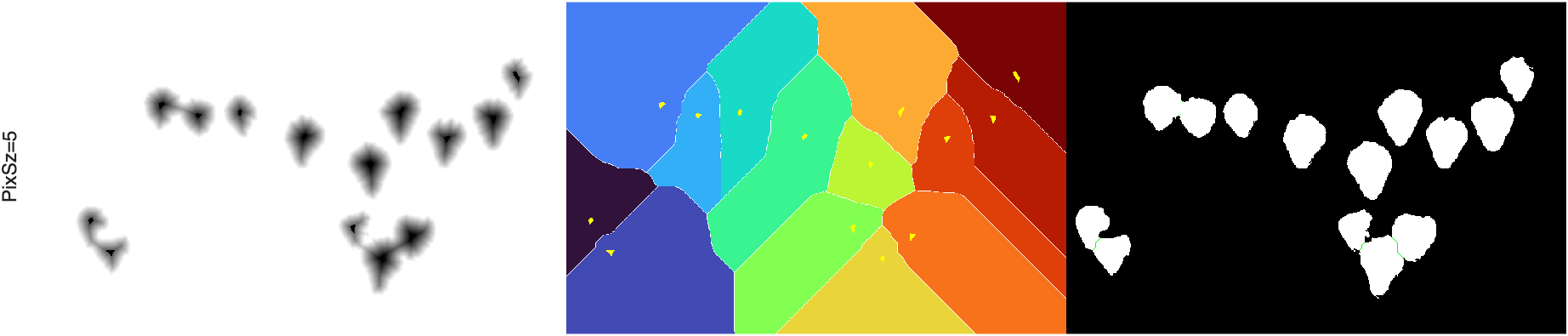
mmGetWatershed with ShowSteps=true, applied to the strawberry mask from Color Segmentation. Left: the inverted distance transform, where each strawberry's center is a dark basin. Middle: the watershed regions, with the basins chosen by imextendedmin overlaid in yellow. Right: the mask before and after separation; the green lines are the pixels removed to split touching strawberries.

Choosing the Basin Depth

The second input to mmGetWatershed is the minimum basin depth, measured in pixels of distance. An object is split off from its neighbor only if its center is at least that many pixels farther from the background than the narrowest point of the neck between them. Shallower basins are merged with their neighbors.

• Larger values split fewer objects. They are conservative and keep a single, irregularly shaped object from being cut into pieces (over-segmentation).
• Smaller values split more objects. They separate tightly fused objects, but increase the risk of over-segmentation.

You can also pass a vector of depths to run the watershed several times. For example, mmGetWatershed(BW,[3 2 2]) runs three passes, going from conservative to aggressive: the first pass makes only the obvious splits, and the later passes split the objects that are still fused.

Where the Watershed Is Used in This Course

• Color Segmentation: separating touching strawberries and candies (mmGetWatershed(mask,5))
• Classifying Kidney Tubules (below): separating touching nuclei (mmGetWatershed(nuc.mask,[3 2 2]))
• Volume Segmentation: separating touching bubbles in a 3D volume (mmGetWatershed(Mask,[3 1])). bwdist works the same way in 3D; the depth is simply measured in voxels instead of pixels.

See the mmGetWatershed reference for all of its options.

Example: Classifying Kidney Tubules

Consider this cross-section through kidney tissue:

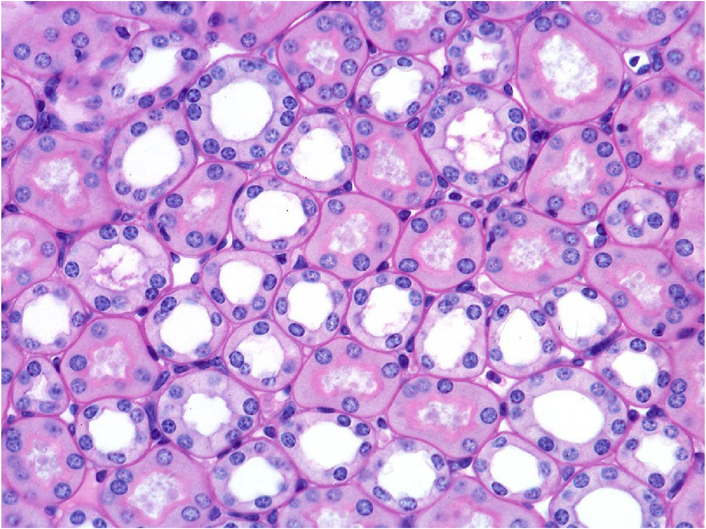
We'll segment the dark nuclei and the white duct lumens, then use the distance transform to figure out which nuclei surround which duct.

Segmenting Nuclei and Ducts

First, a median filter smooths out noise (applied to each color channel separately via the [7 7 1] neighborhood), then we convert to L*a*b* and cluster with imsegkmeans—the same programmatic color segmentation technique from the Color Segmentation module:

p.medf = medfilt3(p.rgb, [7 7 1]);
p.lab = rgb2lab(p.medf);

p.ab = im2single(p.lab(:,:,2:3));
nColors = 4; % white lumen, dark blue nuclei, pink cytoplasm, dark pink
p.label = imsegkmeans(p.ab,nColors, 'NumAttempts',3);

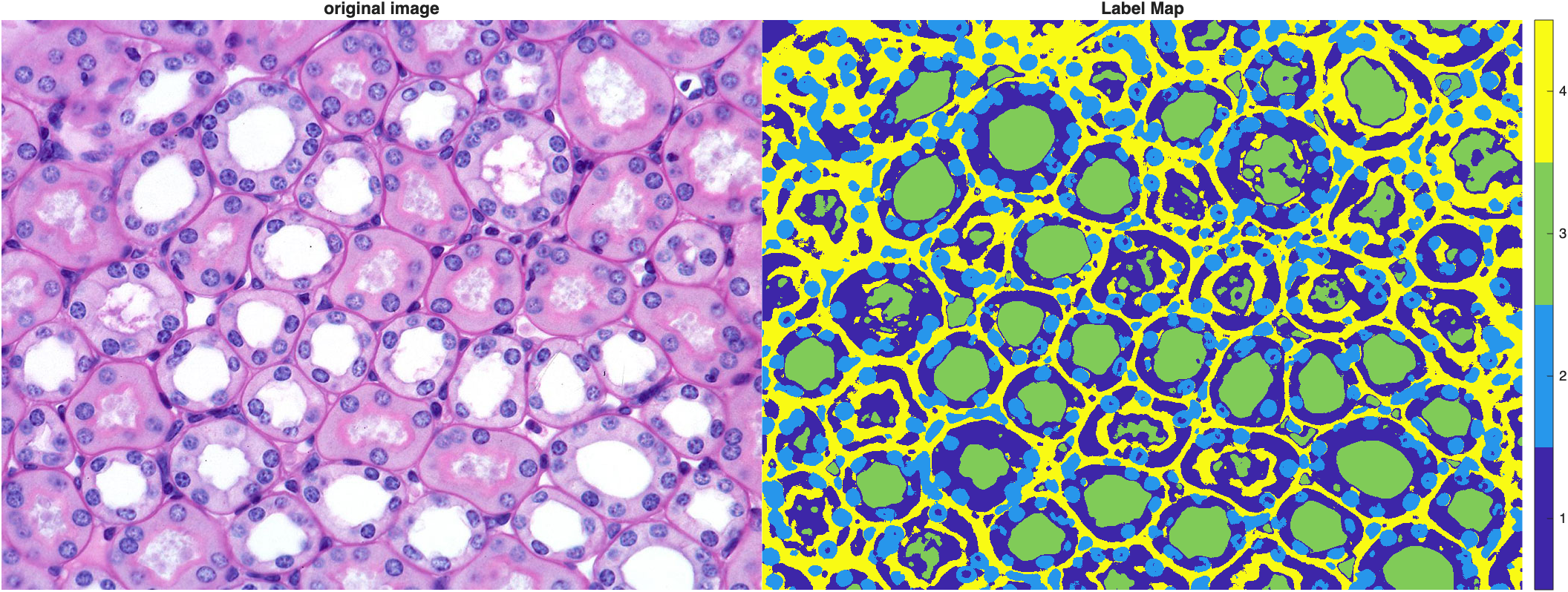
Rather than hard-coding which label number means what—cluster numbers are arbitrary, as we saw in Color Segmentation—we find the nuclei and duct clusters by their lightness (L*): nuclei are the darkest cluster, lumens are the brightest.

rpL = regionprops('table',categorical(p.label),p.lab(:,:,1),'MeanIntensity');

[~, nucLabel] = min(rpL.MeanIntensity); % darkest cluster = nuclei
[~, ductLabel] = max(rpL.MeanIntensity); % brightest cluster = duct lumens

nuc.mask = p.label == nucLabel;

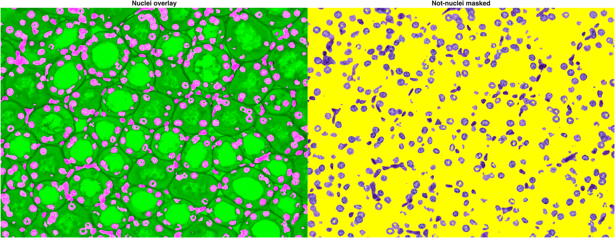
Nice—the nuclei are correctly identified. A standard morphological cleanup (fill holes, remove small noise) followed by a repeated watershed (run three times, with progressively smaller basin depths, to separate touching nuclei) finishes the job:

nuc.mask = imfill(nuc.mask, 'holes');
nuc.mask = bwareaopen(nuc.mask, 50);
nuc.mask = mmGetWatershed(nuc.mask,[3 2 2]);

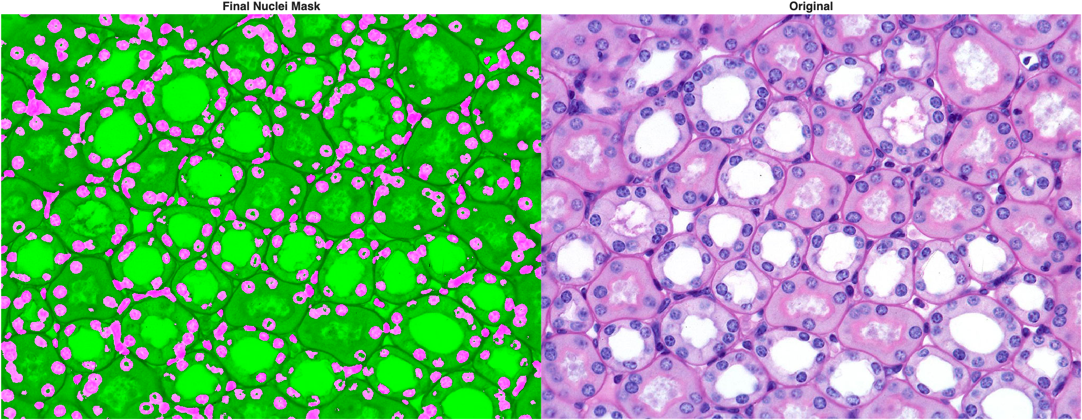
The duct lumens—the brightest cluster—are just as easy to pull out:

duct.maskLAB = p.label == ductLabel;
duct.maskLAB = bwareaopen(duct.maskLAB,1000);

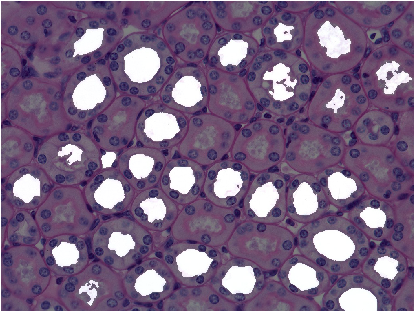
Many of the ducts are captured well, but notice we miss the ones with pink-stained material inside the lumen—their interior isn't part of the "brightest" cluster, so k-means alone can't recover them.

Recovering missed ducts with SAM

The Segment Anything Model (SAM), available through imageSegmenter or the segmentAnythingModel function, can recover ducts that k-means misses, by feeding it the k-means duct and nuclei centroids as foreground and background points respectively (via regionprops). SAM's first run on an image is slow—it has to compute image embeddings, a compact numerical summary—but after that, segmenting with different points is fast. Since it requires the separate Image Processing Toolbox Model for Segment Anything Model support package and a one-time model download, this module continues with the k-means-only duct mask, which is enough to demonstrate the distance transform.

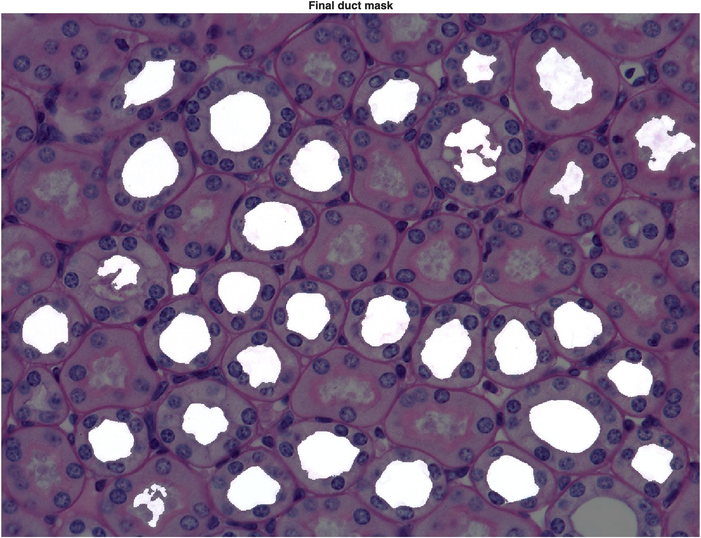
A light morphological cleanup—fill holes, discard any duct touching the image border (a partial duct would give a bad measurement), and discard tiny leftover noise—gives us the final duct mask:

duct.mask = imfill(duct.maskLAB,'holes');
duct.mask = imclearborder(duct.mask);
duct.mask = bwareaopen(duct.mask,750);

How Far Apart Are the Ducts?

With a duct mask in hand, we can use the distance transform to estimate the typical spacing between ducts:

distTxfm = bwdist(duct.mask);
imshow(distTxfm,[])

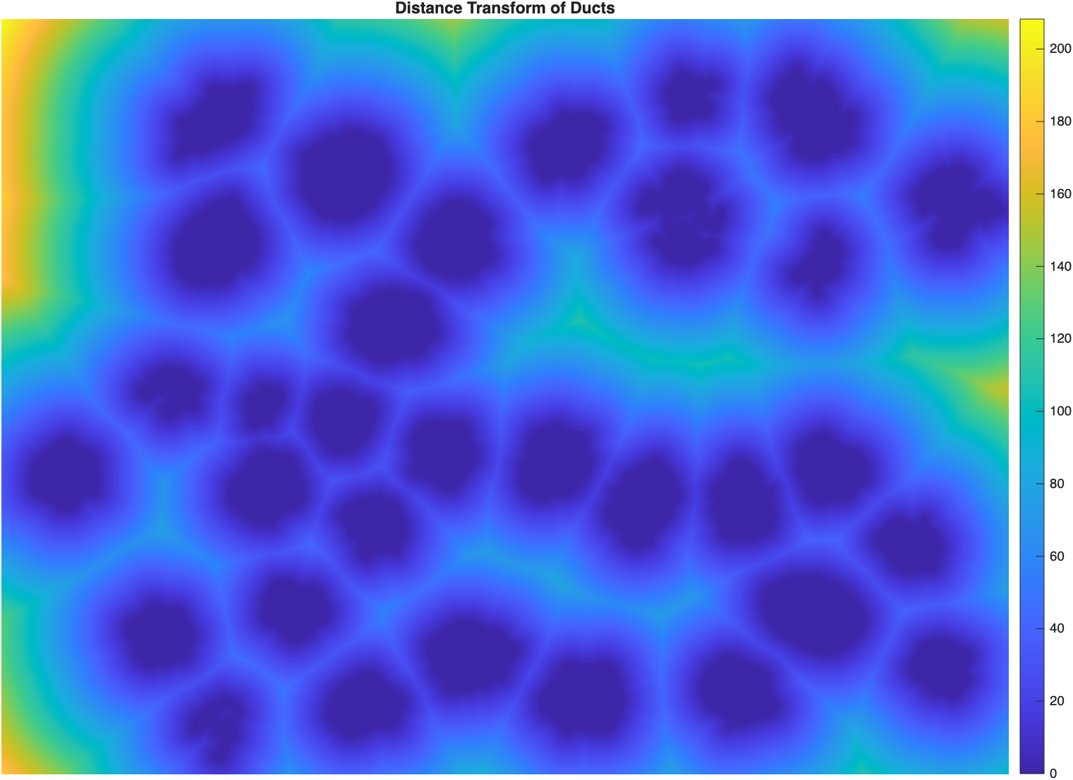
This is exactly the same squircle-tessellation pattern from the four-point toy example above, now shaped by 32 real ducts instead of 4 synthetic points. The ridges (bright lines) mark the halfway points between neighboring ducts.

imregionalmax finds those ridges directly—pixels whose distance value is higher than every one of their immediate neighbors:

regMax = imregionalmax(distTxfm);

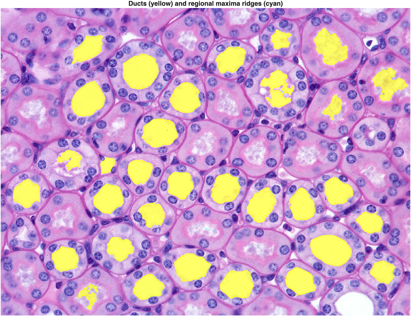
Doubling the distance at each ridge pixel (since a ridge marks the halfway point) gives us a distribution of duct-to-duct separations:

separation = distTxfm(regMax) * 2;
histogram(separation)
title(sprintf('Median Separation = %1.2f',median(separation)))

result

Median Separation = 78.05

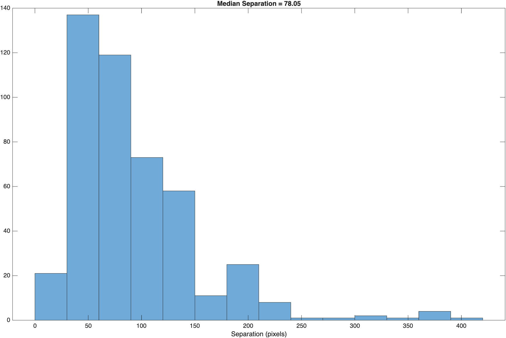
The distribution is right-skewed—a median is a more robust summary here than a mean would be.

Drawing a Boundary Around Each Duct

Now the main event. Why we need the distance transform: if we threshold the distance transform of the duct mask, every pixel between two chosen distances forms a ring around each duct. Nuclei that touch that ring belong to that duct. First, a label map, so we can work with one duct at a time:

duct.label = bwlabel(duct.mask);
max(duct.label(:)) % 32

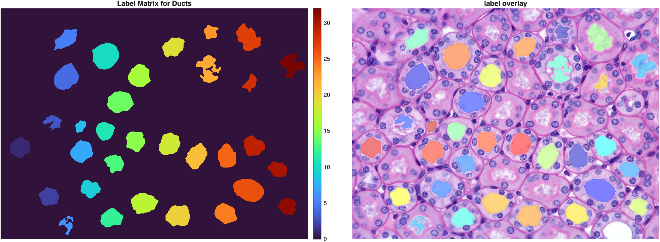
How wide should the ring be? A good width is about one nucleus diameter—wide enough to touch the nuclei lining the duct, but narrow enough to exclude the nuclei of neighboring ducts. The nuclei we already segmented give us a sense of scale:

Typical nucleus size

groupsummary(nuc.rp,[],["mean","std"],"EquivDiameter")

result

mean_EquivDiameter = 18.24    std_EquivDiameter = 10.17

Roughly 18 pixels on average—so a boundary width of 20 pixels is a reasonable starting point. Visualizing the distance transform of just one duct makes the ring concept concrete:

ductID = 15;
duct.mask1 = duct.label == ductID;
duct.distTxfm1 = bwdist(duct.mask1);

imshowpair(duct.mask1,p.rgb,'blend');
hold on
imcontour(duct.distTxfm1,'c-'); % cyan contour lines

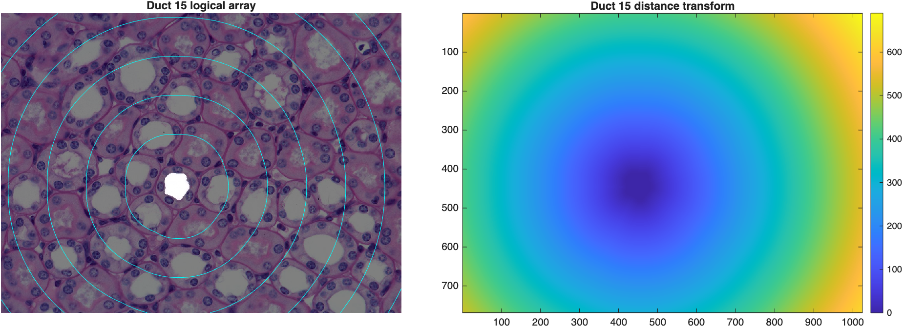
Inside the duct mask itself, the distance transform is zero; the contour lines radiate outward in concentric rings, exactly like the toy examples above.

Thresholding the distance transform between 0 and 20 (excluding 0, which is the duct itself) produces the ring:

duct.distTxfm = bwdist(duct.mask);
duct.boundary = duct.distTxfm > 0 & duct.distTxfm < 20;

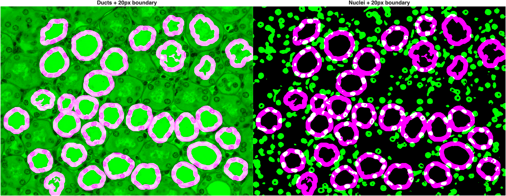
Optimally, the rings shouldn't overlap too much, and should touch—without necessarily fully enclosing—the nuclei that line each duct.

Capturing the Surrounding Nuclei

A ring tells us where to look, but we still need to select the whole nuclei it touches—not just the sliver of each nucleus that happens to fall inside the ring. imreconstruct(marker, mask) keeps every object in mask that touches marker, in full, and drops the rest. Here, the ring is the marker and the nuclei mask is the mask to reconstruct from:

boundaryMask1 = duct.distTxfm1 < 20 & duct.distTxfm1 > 0; % ring around duct 15
BWencircling = imreconstruct(boundaryMask1, nuc.mask);

cc = bwconncomp(BWencircling);
cc.NumObjects % 7

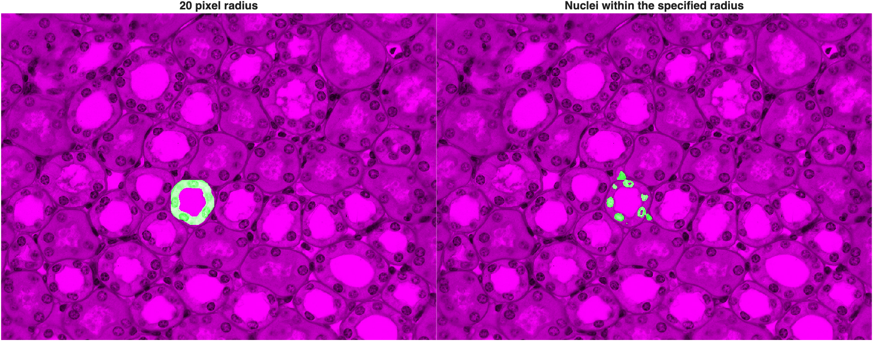
bwconncomp is a quick way to count distinct objects in a mask—NumObjects is the count, and PixelIdxList holds the linear indices of each one.

Looping this process over every duct (with a for loop, iterating over each duct's label) gives us a nuclei count per duct, and labels each set of surrounding nuclei to match its duct:

boundaryWidth = 20;
nuc.label = zeros(size(duct.label),'like',duct.label);
nuc.count = zeros(max(duct.label(:)),1);

for n = 1:max(duct.label(:))
    Dn = bwdist(duct.label == n);
    boundaryMask = Dn < boundaryWidth & Dn > 0;

    BWencircling = imreconstruct(boundaryMask, nuc.mask);
    cc = bwconncomp(BWencircling);

    nuc.count(n) = cc.NumObjects;
    nuc.label(BWencircling) = n; % match nuclei label to duct label
end

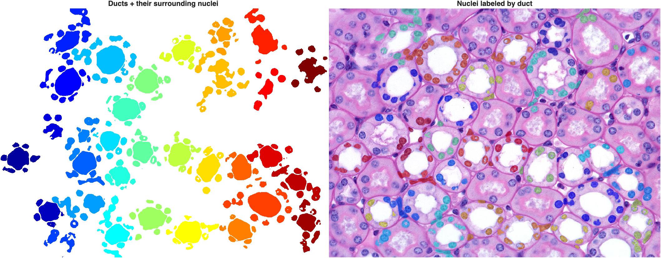
Nuclei counts per duct ranged from 2 to 10 in this image. A nucleus sitting between two ducts touches both rings and gets counted for both—but in the label map, it keeps only the label of whichever duct it was assigned to last in the loop.

Classifying the Ducts

Larger ducts have longer perimeters, so they'll touch more nuclei no matter what type they are. To compare ducts fairly, we normalize the nuclei count by each duct's perimeter:

ductStats = regionprops("table", duct.label, "Centroid","Perimeter", "Area");
ductStats.NucleiCount = nuc.count;
ductStats.NucleiPer100px = 100 * ductStats.NucleiCount ./ ductStats.Perimeter;

histogram(ductStats.NucleiPer100px)
xlabel("Nuclei per 100 px of perimeter")

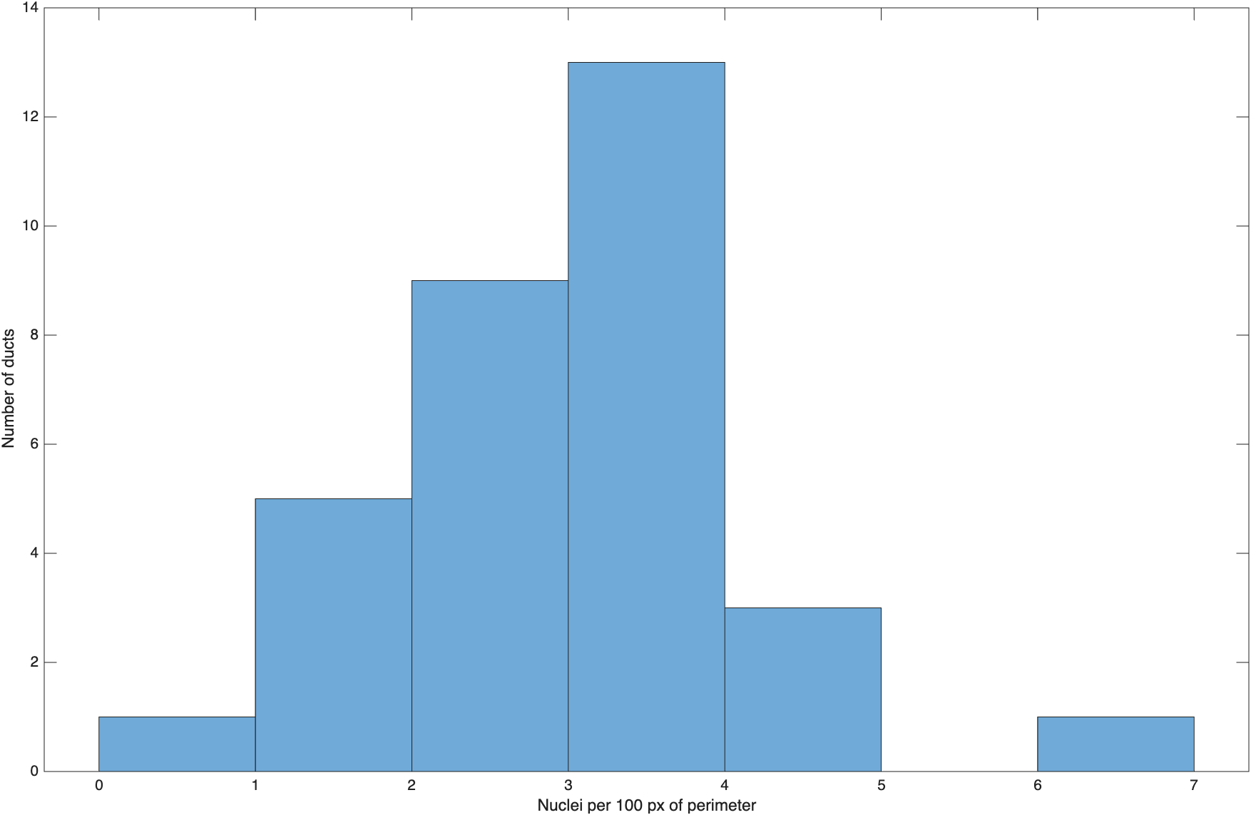
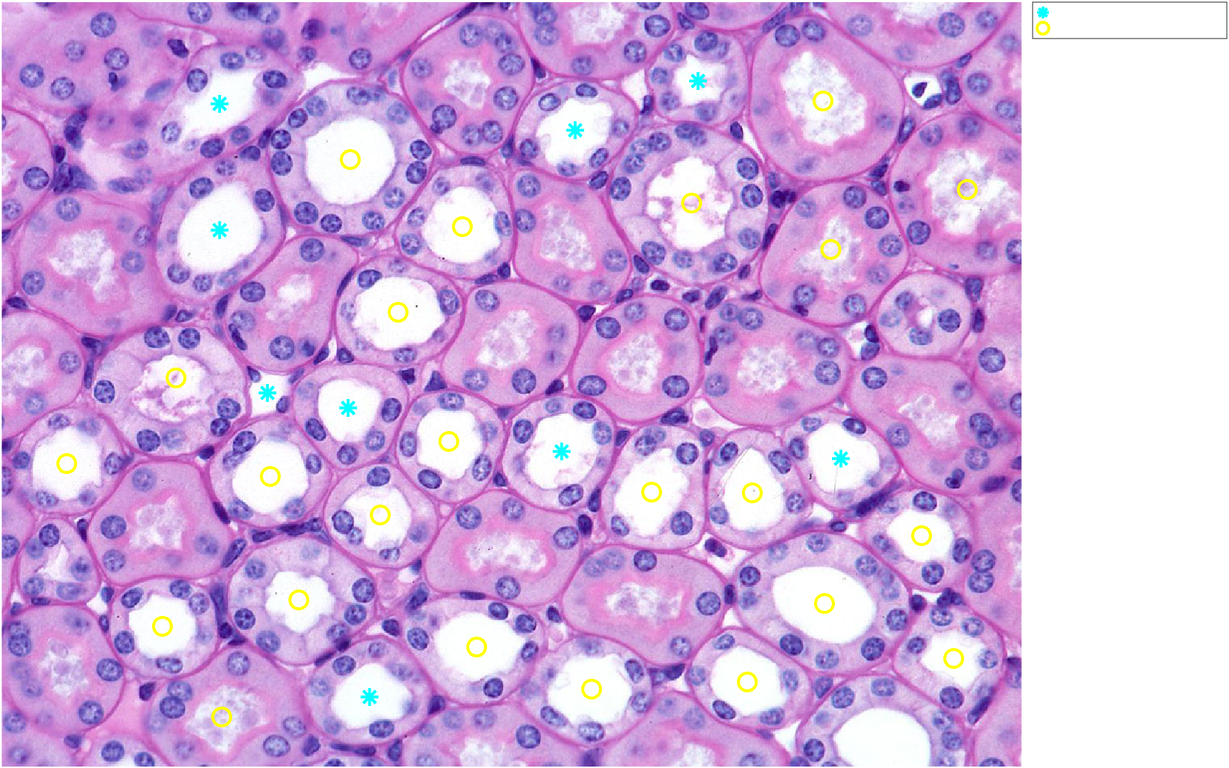
Unlike the earlier toy examples, real tissue doesn't always split as cleanly as we'd like—this distribution is right-skewed with a single high outlier, but no sharp gap separating two obvious groups. That's a realistic result, not a failure: some ducts are irregular or ambiguous (their mask doesn't follow the lumen edge precisely, which throws off both the perimeter and which nuclei the ring happens to touch), and a single global ring width can't be perfectly tuned for every duct's size and shape. Picking a cutoff here (for example, labeling anything above roughly 3.5 nuclei per 100 px as a likely collecting duct) is a judgment call, not something the data hands you automatically—exactly the kind of "the algorithm gives you a number, you still have to interpret it" lesson from Color Segmentation.

Summary

• bwdist gives every pixel its distance to the nearest TRUE pixel in a reference mask.
• Thresholding a distance transform draws a ring (or a disk) of any width around a mask.
• imregionalmax finds the ridges exactly halfway between objects—useful for estimating spacing.
• imreconstruct keeps whole objects that touch a marker, rather than just the pixels that happen to overlap it.
• Normalizing a count by a size measurement (like perimeter) makes comparisons fair across objects of different sizes.

Challenge

How much does the ring width change the nuclei count?

QuestionAnswer

We chose a boundary width of 20 pixels because it's close to the average nucleus diameter. Using duct 15 from this module, try boundary widths of 10 and 30 pixels instead of 20. How does the nuclei count change, and why?

for bw = [10 20 30]
    boundaryMaskBW = duct.distTxfm1 < bw & duct.distTxfm1 > 0;
    enc = imreconstruct(boundaryMaskBW, nuc.mask);
    cc = bwconncomp(enc);
    fprintf('boundaryWidth=%d -> nuclei found: %d\n', bw, cc.NumObjects);
end

result

boundaryWidth=10 -> nuclei found: 6
boundaryWidth=20 -> nuclei found: 7
boundaryWidth=30 -> nuclei found: 12

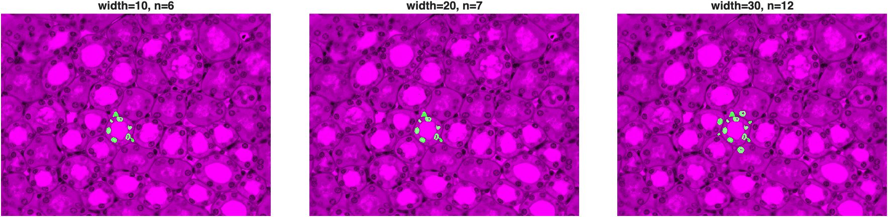
A narrower ring (10 px) barely grazes the inner nuclei and can miss some entirely. The 20 px ring—our original choice—cleanly captures the full ring of nuclei lining the duct. At 30 px, the ring has grown wide enough to start reaching into the next tier of nuclei, and even nuclei belonging to a neighboring duct, nearly doubling the count. There's nothing special about 20; it's a reasonable choice for this image's magnification and nucleus size, not a universal constant—exactly the kind of parameter the summary at the end of Color Segmentation warned about.

Congratulations, you have made it to the end! 📏