MtM Toolbox

The MtM toolbox is a collection of functions designed to simplify Plotting, Image Processing, Processing 3D Slicer segmentation volumes, working with Surface Meshes, and several other utility actions. These functions can be found in the MtMresouces/toolbox folder.

The MtM toolbox folder must be added to search path for these functions to work

Add the MtMresouces/toolbox folder to the MATLAB search path as described on the setup page.

Most MtM toolbox functions are prefaced with mm

You can get a quick summary of the available course functions in the MtMtoolbox by entering help MtMtoolbox in the command window.

Plotting Functions

mmShowHist

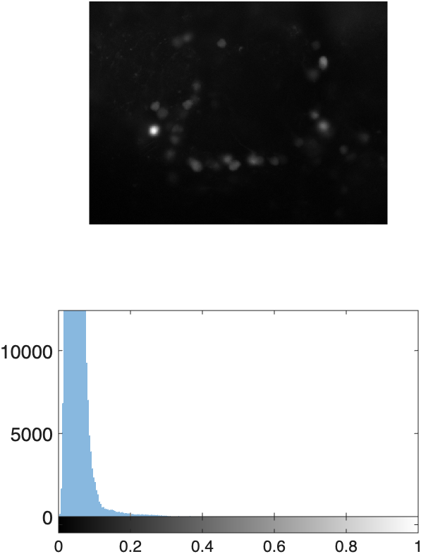
Tiles an image with its histogram in one figure. Image is display above the histogram (two row tiles per image). Corrects MATLAB inexplicable inability to pair nexttile with imhist by using subplot for tiling.

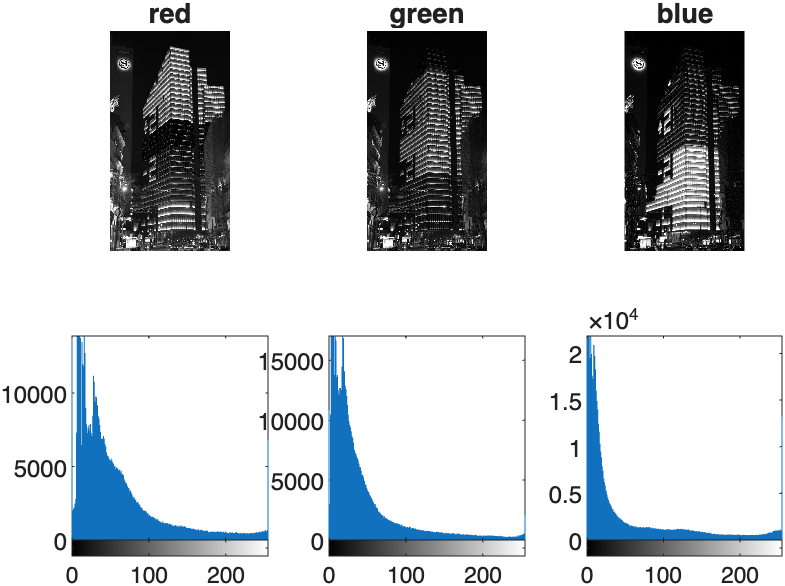
If you input an RGB image, this function will automatically index out the channels and display the histogram for each channel.

INPUTS

Required:

• img: an image matrix

Optional:

• col (default = 1): current column position
• num_cols (default = 1): total number of columns in the figure.
• title_str (default = empty): a string to title the image
• add_color (logical = false): if true add color

mmShowHist(img) — displays image above its histogram
mmShowHist(img, 2, 6) - displays the image and the histogram in the 2nd
column of a six-column figure

mmShowBurnImage

Burns a mask onto an image. Wrapper for imoverlay but with syntax similar to imshowpair.

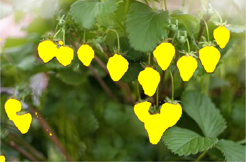
INPUTS

• img: a grayscale or rgb image
• mask: a binary mask

OPTIONAL INPUTS

• color: the color of the burned image (default = yellow)

mmShowBurnImage(rgb,mask)
mmShowBurnImage(rgb,mask,color='white')

mmShowStruct

Displays any images packaged in a structure as a tiled figure. Useful for reviewing image processing steps.

INPUTS

• S: a structure contain fields with image variables
• fn2display: cell array or string array specifying the structure field names to display
• titles (optional): string array of titles for plots

mmShowStruct(p)
mmShowStruct(p,fn2display={'rgb','gray'})
mmShowStruct(p,fn2display={'rgb','gray'},titles={'Original','Grayscale'})

mmBoxSwarm

A wrapper for swarmchart and boxchart that overlays a swarm chart on a box chart.

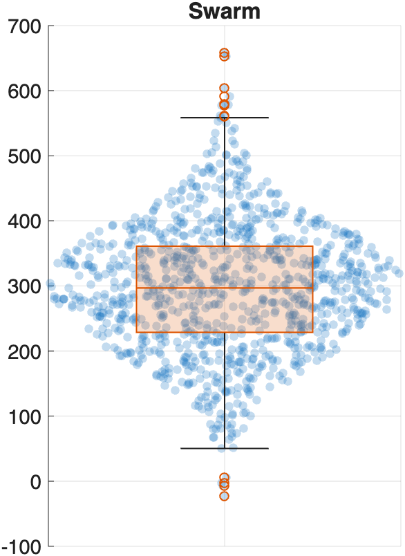
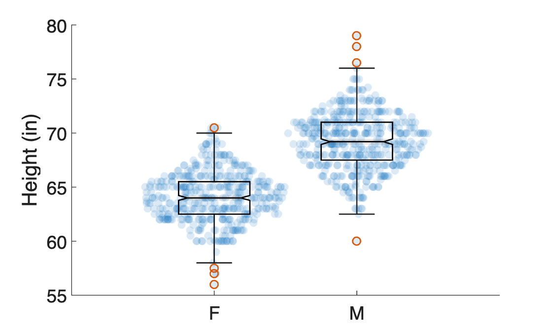
INPUTS

• x: (Optional) Enter empty brackets to generate a series of ones
• y: Vector of numeric data

OPTIONAL INPUTS

• PlotType: enter 'violin' for a violin plot (default is 'swarm')
• XAxVisible: display x-axis (default = 'off')
• MarkerFaceColor: set marker face color
• MarkerFaceAlpha: set marker face alpha (default =0.25)
• doBoxPlot: overlay boxplot (default is true)
• BoxFaceColor: set boxplot face color
• BoxFaceAlpha: set boxplot face alpha (default = 0.1)
• Notch: Turn on box plot notch (default = 'off')
• XJitterWidth: set jitter width of swarm chart (default = 1)

mmBoxSwarm([],nD.data); % y-data only
mmBoxSwarm(x,y,'BoxFaceColor','k','Notch','on','MarkerFaceAlpha',0.15) % grouping data and y-data

mmAddScaleBar

Adds a scalebar to current image

INPUTS

• ax: the handle to the axis where you want to add your scale bar
• width: the length of the scalebar
• widthPERpixel: the dimensions of a pixel side (e.g. um per pixel)

OPTIONAL INPUTS

• Color: the color of the scale bar
• LineThickness: thickness of the scale bar (in points)
• pos: a row vector containing the X and Y coordinates where you want the scale bar. You can enter empty brackets to skip
• unit: a character array indicating the unit of measure. If inputted, the width of the scalebar will be printed above the bar

mmAddScaleBar(gca,100, 2.3);
mmAddScaleBar(gca,50,0.23,'white', 4, [],'µm');

NOTE: the measurements don't have to be in microns. They just have be consistent between width and widthPERpixel

mmHistColor

Overlays the RGB channel histograms of a color image, as either an area plot or a stem plot.

INPUTS

• RGB: an RGB image

OPTIONAL INPUTS

• Pass 'stem' as the second argument to plot the histograms as stem plots instead of the default area plot
• Pass a numeric value below 1 as the second argument to set the fill transparency (alpha) of the area plot (default = 0.75)

mmHistColor(RGB) % area plot of each channel's histogram (default)
mmHistColor(RGB,'stem') % stem plot of each channel's histogram
mmHistColor(RGB,0.4) % area plot with alpha set to 0.4

mmTightTiledLayout

Creates a new figure with a horizontal tiled layout that has no tile spacing or padding.

mmTightTiledLayout
nexttile; imshow(img1)
nexttile; imshow(img2)

Image Processing

mmGetWatershed

Performs the necessary steps for the watershed transformation of a mask. Based on this MATLAB blog

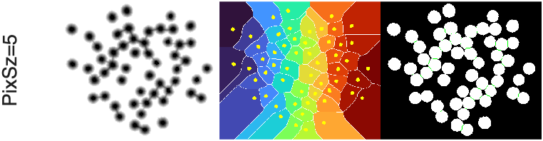
INPUTS

• BW: logical array (2D or 3D)
• PixSz: Pixel Size of the extended regional minima inside the blobs being separated. The smaller the value, the smaller the extended regional minima - see imextendedmin

OPTIONAL INPUTS

• conn: connectivity - see imextendedmin
• ShowSteps: boolean - display watershed steps

OUTPUT

• BW: Watershed transformed Mask

BW = mmGetWatershed(BW,5);
BW = mmGetWatershed(BW,5,ShowSteps=true); % displays transformation steps
BW = mmGetWatershed(BW,5,8); % pixel size 5, connectivity 8
BW = mmGetWatershed(BW,[5 3 1]);  % runs the watershed 3 times with 3 different pixel sizes

mmGetTextureFilters

Applies multiple texture filters to input image. Texture filters include standard deviation, range, and entropy.

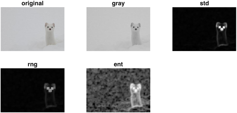
Text Filters applied to an image of a Ferret and displayed using mmShowStruct

INPUTS

• p: a structure that must contain a field called either 'rgb' or 'img'. rgb should be an rgb image. img should be a grayscale image.

• nhood: (optional) a neighborhood matrix (typically logical or array of ones).

OUTPUT

• p: updated structure containing four new fields: gray, std, rng, and ent

p = mmGetTextureFilters(p) % get filtered images with default neighborhood

% Apply a 7x7 neighborhood and display all filtered images
p = mmGetTextureFilters(p,true(7)) % get filtered images with a neighborhood of 7x7
mmShowStruct(p) % display filtered images

mmReadImgND

This function uses the MATLAB Bio-formats toolbox to read in multidimensional image stacks.

REQUIREMENTS

The Bio-formats toolbox, bfmatlab, must be downloaded and added to the search path.

INPUTS (optional)

• file_path is a path to an image file. If you don't input a file path, you will be prompted for a path.

OUTPUTS

• IMGND: an XYZCT multidimensional array
• metadata: the metadata from the array in XML format

[IMGND, metadata] = mmReadImgND(file_path)

mmReadRAWimage

Reads a RAW image (.dng) captured with a Sony DSLR camera.

INPUTS (optional)

• im_file: path to a .dng raw image file. If omitted, you will be prompted to select a file.

OUTPUTS

• RAW: the raw image
• metadata: image metadata (from imfinfo)

[RAW, metadata] = mmReadRAWimage(im_file)

3D Slicer Functions

Functions to process segmentation volumes created in 3D Slicer. Requires the Mathworks Medical Toolbox.

All Slicer volumes should be loaded as medicalVolumes.

mmGetSlicerSegmentInfo

Returns a table containing the properties (e.g. name, color, etc.) of the segmentations found in a seg.nrrd file

INPUTS

• file path to a segmentation file

OPTIONAL INPUTS

• addVolInfo (logical, default = false): include additional volume metadata in the output table

OUTPUT

• a table with segmentation names, layer, label, and color values

segT = mmGetSlicerSegmentInfo(seg_file_path)

mmGetSlicerSegmentInfoAll

Loads the metadata and Segmentation Properties from all Slicer segmentation files found in the same folder

INPUTS

• filePath: file path to the folder containing segmentation files (*.seg.nrrd)

OUTPUT

• T: Slicer Segmentation table. Contains information (name, color) about segmentations created in Slicer Segment Editor module
• contentT: Table containing information about the segmentation files

[segT,contentT] = mmGetSlicerSegmentInfoAll(fullfile(paths.folder, paths.fileWC))

mmGetMedicalVolumeSegment

Indexes out a segment from a Slicer Segmentation volume loaded as a medicalVolume. The function returns a structure that contains the mask of the indicated segment, color, and transformation matrix of the selected segmentation. First load a Slicer Segmentation file using medicalVolume and the Slicer segmentation table using mmGetSlicerSegmentInfo.

INPUTS

• mV (required): medicalVolume of a Slicer Segmentation dataset
• segT (required): table - table created by mmGetSlicerSegmentInfo
• segName (optional): string - Name of Segment to return.

If segName not provided, you will be prompted to select one segmentation from the inputted segT table.

OUTPUTS

S: The function returns a structure with the following fields

• segName: Name of selected segment
• mask: binary mask of the selected segment
• color: color of the segmentation as set in Slicer
• tform: transformation matrix to properly orient segmentation
• spacing: Voxel spacing
• volume: calculated using regionprops3.

S = mmGetMedicalVolumeSegment(mv,segT,segName="right kidney")

mmPlotAllSeg

Wrapper function that plots all segmentations from a 3D Slicer segmentation volume. Options include Smoothing and decimation, and lighting.

INPUTS

• mV: medicalVolume of a Slicer Segmentation dataset
• segT: Table containing the following slicer info — Name, Layer, LabelValue, Color

OPTIONAL INPUTS. Enter empty brackets if skipping.

• new_figure: logical (default = true). Create new figure if true
• falpha: scalar (0-1, default = 0.5) - transparency of the faces
• smooth: boolean (default=false). True means Smooth volume

OUTPUT

• hp: array of patch handles to surface plots

segT = mmGetSlicerSegmentInfo(seg_file);
hp = mmPlotAllSeg(mV,segT);
hp = mmPlotAllSeg(mV,segT, falpha=0.25);

mmVolShowPair

Displays two volshow viewers side-by-side in a tiled layout, for comparing two segmentations. Designed to work with structures returned by mmGetMedicalVolumeSegment.

INPUTS

• seg1, seg2: structures (from mmGetMedicalVolumeSegment) each containing a mask and tform field

OPTIONAL INPUTS

• segTitle: title for the display window (default = "My Seg Comparison")

S1 = mmGetMedicalVolumeSegment(mV,segT,segName="right kidney");
S2 = mmGetMedicalVolumeSegment(mV,segT,segName="left kidney");
mmVolShowPair(S1,S2,"Kidney Comparison")

mmSetVolShowColors

Applies a Medical Colormap and alphamap to a volshow render, and optionally sets the viewer's background color. If no MapName is provided, a selection dialog pops up.

INPUTS

• hVolShow: handle to a volshow object

OPTIONAL INPUTS

• MapName: name of the Medical Colormap to apply. Options: CTBone, CTBoneShift, CTCoronary, CTLung, CTSoftTissue, MRI, PET
• BackgroundColor: background color of the viewer (default = 'white'). Set to 'default' to leave the background unchanged.
• BackgroundGradient: turn on a background gradient (default = 'off')
• GradientColor: color of the background gradient (only applies if BackgroundGradient is on)

OUTPUT

• MapName: name of the colormap that was applied

MapName = mmSetVolShowColors(hVolShow)
MapName = mmSetVolShowColors(hVolShow,MapName="CTLung")

mmSaveViewer3D

Saves a viewer3d figure (e.g. from volshow) to an image file.

INPUTS (optional)

• FigHandle: the uifigure that contains the viewer3d (e.g. hVolShow.Parent)
• Fullpath: file path to save the image to. If omitted, you will be prompted to choose a location.

mmSaveViewer3D(hVolShow.Parent)

Surface Functions

Functions to process and manipulate surface meshes. Many of these functions work well with the vertices field in a patch handle, allowing for real-time update of the surface plot.

mmPlotMask2Surface

Wrapper function that creates an isosurface from an input volume. Options include smoothing of the volume, decimation, and lighting. Default plots surface as a patch in one simple function call.

INPUTS

• BW: logical 3D array

OPTIONAL INPUTS (in this order). Enter empty brackets if skipping.

• fcolor: character array (default = 'cyan') - facecolor of the isosurface.
• falpha: scalar (0-1, default = 0.5) - transparency of the faces
• lightEMup: boolean (default = true) - add lights to the scene. For multiple function calls, set to false for all calls, except the last one. Then set to true on the final call. Otherwise you'll add too many lights to the scene.
• report: boolean (default=false) - print a report of settings to command window
• smooth: boolean (default=false). True means Smooth volume
• decimator: decimation factor (0-1, default=0.15) of the generated surface
• transform: affinetform3d 3D affine transformation (default = no transformation). Used to transform the vertices to match the orientation and size of the original volume.

OUTPUT

• hp: handle to patch

hp = mmPlotMask2Surface(BW);
hp = mmPlotMask2Surface(BW,fcolor='cyan');
hp = mmPlotMask2Surface(BW,fcolor='magenta',falpha=0.25, lightEMup=true, decimator=0.2);

tform = createScaling3d(Sseg.xyz)
hp = mmPlotMask2Surface(BW,'magenta',transform=tform); 

mmGetSurface

Generate a surface mesh of the inputted 3D volume. Returns a face-vertices structure.

INPUTS

• Vol: a 3D volume
• iv (numeric): isovalue from which to generate the surface
• decimator (0-1): amount by which to decimate the generated surface.
• use_fast_march (logical): Use the function extractIsosurface to more quickly generate an isosurface. Default = true.
• centerSurface (logical): Center the vertices to 0,0,0. Default = false
• transform: affinetform3d 3D affine transformation (default = no transformation)

OUTPUT

• fv: a faces-vertices structure
• s: string reporting the decimation

fv = mmGetSurface(Vol);
fv = mmGetSurface(Vol,0.5,0.1) 

REQUIREMENTS

Medical toolbox required for fast marching isosurface

mmPlotSurface

Wrapper function to patch. plots the input fv structure as a patch. Lights not added. Use mmSetSurfacePlotProps to add lighting and correct aspect ratios

INPUTS

• fv: a faces-vertices structure (output from isosurface)
• fcolor: face color
• falpha: face alpha

OUTPUT

• hp: handle to the patch

hp = mmPlotSurface(fv,'cyan',0.5);
mmSetSurfacePlotProps % add lighting to plot

mmSetSurfacePlotProps

Sets the light position, aspect ratio, and axis labels for a surface plot. Call after mmPlotSurface — or, if plotting multiple surfaces in a loop, call once after the last plot.

No inputs or outputs.

hp = mmPlotSurface(fv,'cyan',0.5);
mmSetSurfacePlotProps

mmAlignSurface2Axes

Transforms the vertices so that the direction of most variance is aligned to the x-axis. Based on this discussion.

INPUTS

• Vert: NX3 array of Vertices to be transformed

OUTPUT

• Vert: Transformed vertices
• Vd: Variance

hp.vertices = mmAlignSurface2Axes(hp.vertices)

mmRotateSurfaceVertices

Rotate the vertices of a surface around the specified axis by the specified angle (in degrees).

INPUTS

• vertices: (matrix): Nx3 vertices
• ax (character array): axis around which to rotate — x, y, or z
• angl (scalar): angle (in degrees) to rotate
• centerVerts (logical): optional. Center Vertices around 0,0,0 prior to rotation

vertices = mmRotateSurfaceVertices(vertices, 'x',45)

mmCreateRotationMat

Creates an affine rotation matrix (affinetform3d) for rotating about the x, y, or z axis. Useful for building a transform to pass into functions like mmPlotMask2Surface or mmGetSurface.

INPUTS

• angl: amount of rotation, in degrees
• ax: axis to rotate around — 'x', 'y', or 'z'

OPTIONAL INPUTS

• origin: 1x3 vector — origin to rotate around (default = [0 0 0])

OUTPUT

• tform: affinetform3d affine rotation transformation

tform = mmCreateRotationMat(45,'x')

mmAlignSurfaces

Registers two point clouds using an iterative closest point algorithm. This function requires the Computer Vision Toolbox. The inputs and outputs of this function are a matrix of 3D coordinate points (xyz)

INPUTS

• vertFixed: NX3 vertices matrix of Fixed Surface
• vertMoving: NX3 vertices matrix of Surface to be moved (registered to fixed surface)

OUTPUT

• vertMoving: NX3 vertices matrix of registered surface
• rmse: root-mean-square error of the final registration

 [vertMoving,rmse] = mmAlignSurfaces(vertFixed, vertMoving,options)

mmCalcSurfaceAreaFromMesh

This function will calculate the sum of all triangles in the mesh to calculate Surface area.

If P1, P2, and P3 are 3D coordinate vectors of the three respective vertices of some particular triangle, then its area is given by:

AreaP1P2P3 = 1/2*norm(cross(P2-P1,P3-P1));

Adapted from this discussion

[SurfaceArea] = mmCalcSurfaceAreaFromMesh(Vertices,Faces)

Apps

mmSliceView

A custom image stack viewer app. Can handle 3D and 4D image stacks. Can load Image Stacks and accompanying binary Masks

Benefits

• Relatively Responsive
• Quickly scrub through image using the mouse scroll wheel
• Turn on image contrast for each slice
• Simultaneously load an image stack and a mask — overlay the mask on each slice view

mmSliceView(STACK)

Utility Functions

mmSetFigPublication

Sets the default axes font to 16 and figure color to white

mmSetFigPublication(14) % Set Font size to 14

mmSetUnitDataFolder

Sets the current folder to the indicated unit data folder from the MtMdata Shared Folder (Must be at root level of MATLAB drive)

mmSetUnitDataFolder(3) % sets folder to unit 3 

mmGetChannelMap

This function returns a color map (with 256 shades) of the indicated color

INPUT: a channel name, letter, or index OUTPUT: a colormap of the shade indicated by the input

red_cm = mmGetChannelMap('red')
green_cm = mmGetChannelMap('g')